
Classification and the DHS
For this project, I wanted to take a deeper dive into an area in which I had subject domain knowledge. As a graduate student of health systems at Johns Hopkins, I frequently used summary stats and figures pulled from the World Bank Indicators Project or the Demographic and Health Surveys, but rarely needed to do any original analyses myself on the rich, raw data underlying these reports. Taking inspiration from a recent publication, I decided to explore the role of child marriage as a predictor of intimate partner violence (IPV) using machine learning classification algorithms.
Definitions, dataset, and methods
For the purposes of this exercise I employed internationally accepted definitions.
Intimate Partner Violence (IPV): “Any behaviour within an intimate relationship that causes physical, psychological, or sexual harm to those in the relationship” – WHO
Child marriage: “A formal marriage or informal union, such as cohabitation, before age 18 or legal age of consent in the country of interest” – UN
In order to create my target variable, I coded a woman as “ever abused by an intimate partner” if she had answered “yes”, “sometimes”, or “often” to any of the multiple questions regarding IPV. It is a common survey technique to ask the same question in multiple specific ways – such as “were you ever kicked”, “were you ever punched” – this is merely a device to improve participant recall.
Since I decided to use the DHS Women’s Recode cross-sectional survey from 2012-2013, I created a dummy variable for whether the woman had been married off as a child, where “yes” meant that she had cohabitated before age 16, which is the age of consent for females in Pakistan.
The DHS is extensive, and given the nature of the question I decided to focus on adding label variables to my model selectively, in particular focusing on features that would likely be confounding factors in a purely statistical model, such as the education of the woman, her household wealth, and her age at time of survey.
I approached the analysis then with two complementary models.
Model I: Determining households with women at risk
The first model assumed a case where we would wish to target households with women potentially at-risk for IPV, such as with an educational campaign disseminating a help-line number to women in need. We are willing to accept false positives more readily than false negatives, as we would like all women at risk to know that a help-line exists. Moreover, it seems reasonable to request that such a campaign would be designed as to not alienate husbands or women who do not experience IPV, and so false positives are not especially concerning, aside from potential misdirection of limited resources.
With this scenario in mind, we optimize our model for recall over precision.
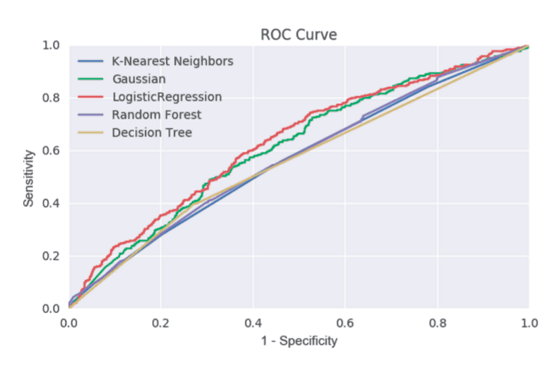
I trained a subset of my data on multiple classification models with scikit-learn, tested each model on a representative hold-out/test set of data, and plotted their resulting Receiver Operating Characteristic, or ROC, curves on the same axes. I found that in most cases Logistic Regression outperformed the other available models.
I then looked at whether I could improve recall by adjusting the threshold. A scikit-learn model will produce probabilities associated with the target to show the model’s uncertainty regarding the classification it has chosen. By default the threshold is 0.5*, meaning that a probability of less than 1/2 will be classified as “no” and above or equal to this threshold would be classified as “yes”.
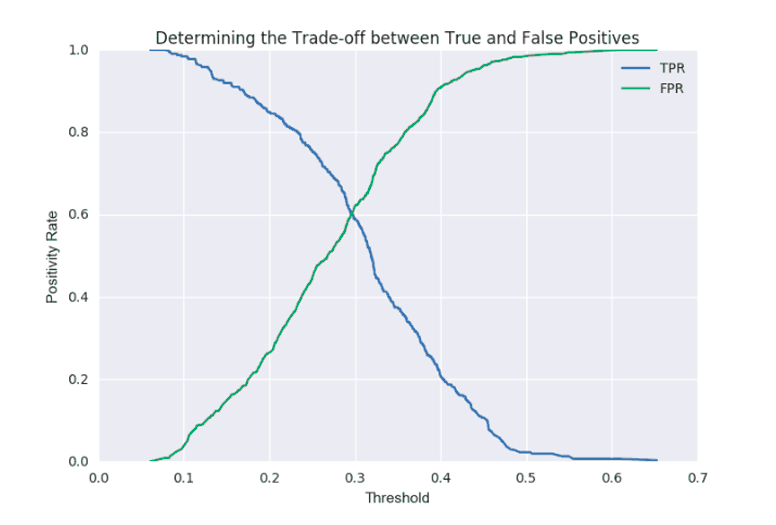
In this particular model, we initially gain precision while also increasing our recall at threshold = 0.3, which is very near the optimization point between false positives and false negatives. With our threshold set, we now have a model which we could use on additional data to classify as households with women at risk for IPV.
Model II: Does child marriage increase risk of IPV?
In the problem statement, however, we were specifically interested in the impact of child marriage as a precondition for IPV. To this end, I wanted to first simplify the model somewhat by taking the label features related to household assets, characteristics, and access to improved WASH facilities and combine them into a handful of few features using Principal Components Analysis (PCA) that capture, in a sense, a more generalized picture of the household’s wealth. PCA has been used successfully as a proxy for socioeconomic status in regions where income is not a straight-forward assessment of individual or household wealth, and in fact the statisticians at DHS create wealth indices to accompany their surveys using PCA and feature weights, but for the purposes of this exercise I will generate my own approximate “wealth” index.
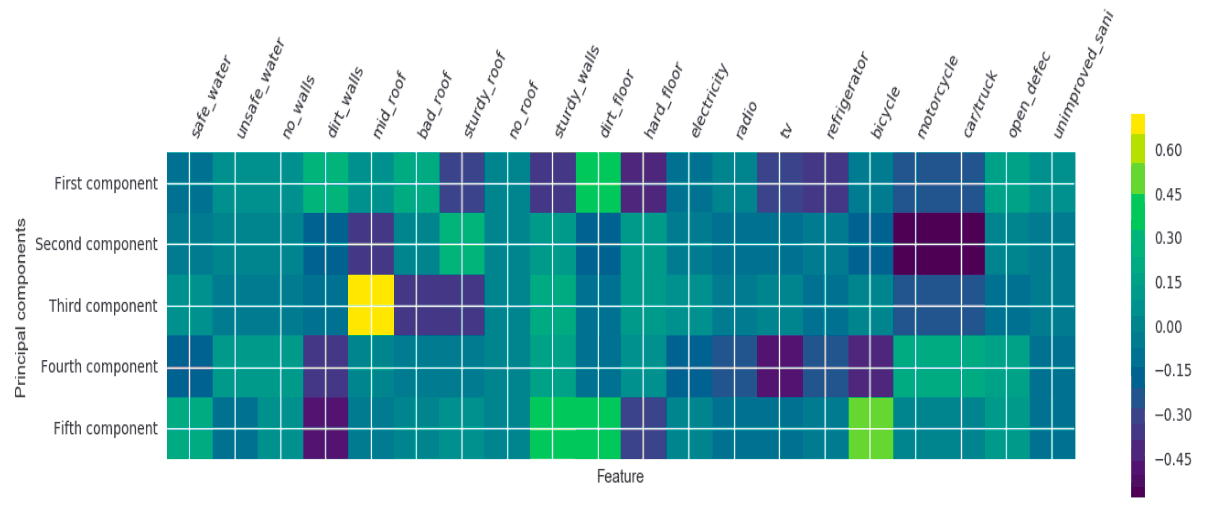
We can see how much each component explains feature variability in order to help determine how many components we will need total. In this case, I settled on compressing 21 household attribute features into five components, which together could explain 60% of the information contained in the full set of 21. I chose five because I wanted explanatory power greater than 50%, and beyond five there were increasingly diminishing returns.
A “good” component feature in the following heatmap is one where each of the features shows up green, or near zero. If we think of PCA as a transformation of axes, we would expect “green” or 0 if our feature’s component lies directly on the transformed vector. A “dark purple” or “bright yellow” indicates greater distance from the vector. In order to improve our “wealth” index, we could consider adding or subtracting features, or look to future surveys which may obtain actual costs of household assets, which may allow the model to perform better.
Finally, I ran a logistic regression with and without child marriage using statsmodels.api and found that the coefficient for child marriage was 0.3129. Since under the hood logistic regression is just the same as linear regression after taking the ln (log base e) in order to make the function continuous, we can obtain an odds ratio by simply raising e to the power of the coefficient, which in this case gives us 1.367. A one-unit increase therefore between u16_marriage (where 0 = no and 1 = yes) increases the odds of “ever IPV” by 37% with statistical significance (p=0.001), all other things being equal.
View my code
You can find my code, as well as presentation slides, on Github.
Notes
*This is not strictly true, which you can examine by printing out all the probabilities and the model’s associated classification for each, but in this case it is an adequate heuristic for understanding the basic logic of my model design.