Survival Analysis to Explore Customer Churn in Python
Originally posted in the online publication “Towards Data Science” on Medium
Survival analysis refers to a suite of statistical techniques developed to infer “lifetimes”, or time-to-event series, without having to observe the event of interest for every subject in your training set. The event of interest is sometimes called the subject’s “death”, since these tools were originally used to analyze the effects of medical treatment on patient survival in clinical trials.
Meanwhile, customer churn (defined as the opposite of customer retention) is a critical cost that many customer-facing businesses are keen to minimize. There is no silver bullet methodology for predicting which customers will churn (and, one must be careful in how to define whether a customer has churned for non-subscription-based products), however, survival analysis provides useful tools for exploring time-to-event series.
Why can’t we just use OLS linear regression?
OLS works by drawing the regression line that minimizes the sum of the squared error terms. With unobserved data, however, the error terms cannot be known, and therefore it would be impossible to minimize these values.
Simply taking the date of censorship to be the effective last day known for all subjects, or worse dropping all censored subjects can bias our results.
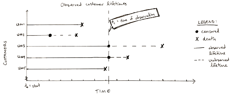
In the graphic above, U002 was censored from loss to follow-up (perhaps due, for example, to an unresolved technical issue on the account that left the customer’s status unknown at the time of the data pull), and U003 and U004 are censored because they are current customers. As of t1, only U001 and U005 have both observed birth and death. As the graphic makes clear, dropping unobserved data would under-estimate customer lifetimes and bias our result.
Survival analysis handles event censorship flawlessly. A customer who has been censored is one whose death has not been observed. The main way this could happen is if the customer’s lifetime has not yet completed at the time of observation. (N.B. In clinical trials, patients who have been lost to follow-up or dropped out of the study are also considered censored.)
Kaplan-Meier curves
For any problem where every subject (or customer, or user) can have only a single “birth” (enrollment, activation, or sign-up) and a single “death” (regardless of whether it is observed or not), the first and best place to start is the Kaplan-Meier curve. This will allow us to estimate the “survival function” of one or more cohorts, and it is one of the most common statistical techniques used in survival analysis.
Survival analysis can be used as an exploratory tool to compare the differences in customer lifetime between cohorts, customer segments, or customer archetypes. In Python, we can use Cam Davidson-Pilon’s lifelines library to get started.
Take, for example, this IBM Watson telco customer demo dataset. By segmenting on the binary feature for single versus multiple phone lines, we get the following Kaplan-Meier curves.
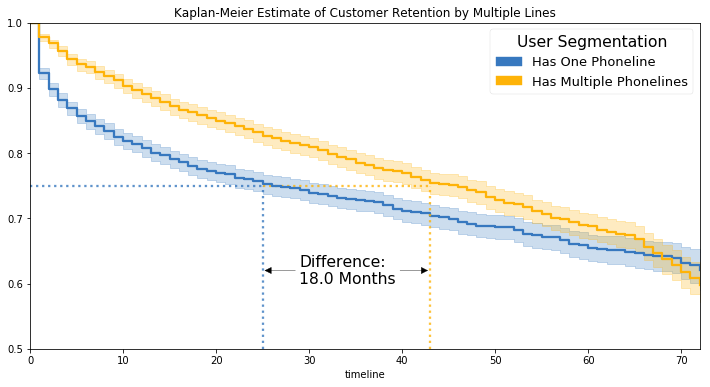
We can see that 1 in 4 users have churned by month 25 of those who have only one phone line. By comparison, 1 in 4 users churn by month 43 among those with multiple phone lines, for a difference of 18 months (an extra 1.5 years of revenue!)
Correlation is not causation, and therefore this graph alone cannot be considered “actionable”. We may, however, look at this and begin to suspect some possibilities, such as that customers with multiple phone lines are more “locked in” and therefore less likely to churn than single phone line users. On the other hand, perhaps customers who are more loyal tend to prefer multiple phone lines in the first place.
And who should get more investment? If the two groups are equally profitable, it may be worth spending more to keep the single phone line users happy, since they currently tend to churn more quickly. Or, an experimental design could reveal that some incentives double lifetimes for all customers, and since the lifetimes of multiple line users tend to be longer originally, this multiplying effect actually would be more profitable for that segment.
Without more context, and possibly experimental design, we cannot know for sure.
Pros and Cons of Kaplan-Meier Curves
Pros:
- Minimal feature set needed. Kaplan-Meier only needs the time which event occurred (death or censorship) and the lifetime duration between birth and event.
- Many time-series analyses are tricky to implement. Kaplan-Meier only needs all of the events to happen within the same time period of interest
- Handles class imbalance automatically (any proportion of deaths-to-censored events is okay)
- Because it is a non-parametric method, few assumptions are made about the underlying distribution of the data
Cons:
- Cannot estimate the magnitude in difference of the survival-predictor relationship of interest (no hazard ratio or relative risk)
- Cannot account for multiple factors simultaneously for each subject in the time to event study, nor control for confounding factors
- Assumes independence between censoring and survival, meaning that at time t, those who have been censored should have the same prognosis as those who have not been censored.
- Because it is a non-parametric model, it is not as efficient or accurate as competing techniques on problems where the underlying data distribution is known
Now try it yourself!
To see how I made this Kaplan-Meier plot and to get started with your own survival analysis, download the jupyter notebook from my Github account.